17_R
- hrafnulf13
- Nov 17, 2020
- 6 min read
Updated: Nov 19, 2020
1.
The law of large numbers is one of the most important theorems in probability theory. It states that, as a probabilistic process is repeated a large number of times, the relative frequencies of its possible outcomes will get closer and closer to their respective probabilities.
For example, flipping a regular coin many times results in approximately 50% heads and 50% tails frequency, since the probabilities of those outcomes are both 0.5.
This figure is example from homework application (p = 0.5, epsillon = 0.1).

Formula for LLN:

n is the number of times the random process was repeated.
Nn(outcome) is the number of times a given outcome has occurred after n repetitions.
P(outcome) is the probability of the outcome.
For any given n, Nn(outcome)/n equals the relative frequency of that result after n repetitions.
Weak and Strong laws [2]:
Weak law states that the sample average converges in probability towards the expected value. Weak law states that for any nonzero margin specified, no matter how small, with a sufficiently large sample there will be a very high probability that the average of the observations will be close to the expected value; that is, within the margin.
Strong law states that the sample average converges almost surely to the expected value. This means is that the probability that, as the number of trials n goes to infinity, the average of the observations converges to the expected value, is equal to one.
2.
Binomial distribution can be thought of as simply the probability of a SUCCESS or FAILURE outcomes in an experiment that is repeated multiple times [3]. The binomial is a type of distribution that has two possible outcomes. For example, a coin toss has only two possible outcomes: heads or tails and taking a test could have two possible outcomes: pass or fail.

The first variable in the binomial formula, n, stands for the number of times the experiment runs.
The second variable, p, represents the probability of one specific outcome.
For example, let’s suppose you wanted to know the probability of getting a 1 on a die roll. if you were to roll a die 20 times, the probability of rolling a one on any throw is 1/6. Roll twenty times and you have a binomial distribution of (n=20, p=1/6). SUCCESS would be “roll a one” and FAILURE would be “roll anything else". If the outcome in question was the probability of the die landing on an even number, the binomial distribution would then become (n=20, p=1/2). That’s because your probability of throwing an even number is one half.
Binomial distributions must also meet the following three criteria:
The number of observations or trials is fixed. In other words, you can only figure out the probability of something happening if you do it a certain number of times. This is common sense—if you toss a coin once, your probability of getting a tails is 50%. If you toss a coin a 20 times, your probability of getting a tails is very, very close to 100%.
Each observation or trial is independent. In other words, none of your trials have an effect on the probability of the next trial.
The probability of success (tails, heads, fail or pass) is exactly the same from one trial to another.
The binomial distribution formula is:

3.
The de Moivre–Laplace theorem, which is a special case of the central limit theorem, states that the normal distribution may be used as an approximation to the binomial distribution under certain conditions [6]. In particular, the theorem shows that the probability mass function of the random number of “successes” observed in a series of n independent Bernoulli trials, each having probability p of success (a binomial distribution with n trials), converges to the probability density function of the normal distribution with mean np and standard deviation sqr(np(1-p)), as n grows large, assuming p is not 0 or 1.

4.
The central limit theorem (CLT) establishes that, in many situations, when independent random variables are added, their properly normalized sum tends toward a normal distribution (informally a bell curve) even if the original variables themselves are not normally distributed [4]. The theorem is a key concept in probability theory because it implies that probabilistic and statistical methods that work for normal distributions can be applicable to many problems involving other types of distributions.
Let X1, …., Xn be a sequence of independent and identically distributed random variables drawn from a distribution of expected value given by μ and finite variance given by σ². We take the sample average of these variables:

According to the LLN, this converges in probability and almost surely to μ when n approaches infinity.

Whatever the form of the population distribution, the sampling distribution tends to a Gaussian, and its dispersion is given by the Central Limit Theorem.
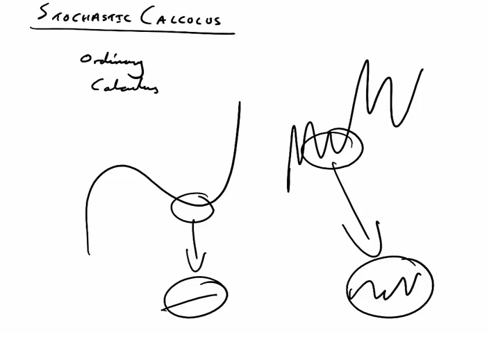
5.
A stochastic or random process can be defined as a collection of random variables that is indexed by some mathematical set, meaning that each random variable of the stochastic process is uniquely associated with an element in the set [5]. The set used to index the random variables is called the index set. Historically, the index set was some subset of the real line, such as the natural numbers, giving the index set the interpretation of time. Each random variable in the collection takes values from the same mathematical space known as the state space. This state space can be, for example, the integers, the real line or n-dimensional Euclidean space. An increment is the amount that a stochastic process changes between two index values, often interpreted as two points in time. A stochastic process can have many outcomes, due to its randomness, and a single outcome of a stochastic process is called, among other names, a sample function or realization.
A stochastic process can be classified in different ways, for example, by its state space, its index set, or the dependence among the random variables. When interpreted as time, if the index set of a stochastic process has a finite or countable number of elements, such as a finite set of numbers, the set of integers, or the natural numbers, then the stochastic process is said to be in discrete time. If the index set is some interval of the real line, then time is said to be continuous. The two types of stochastic processes are respectively referred to as discrete-time and continuous-time stochastic processes. Discrete-time stochastic processes are considered easier to study because continuous-time processes require more advanced mathematical techniques and knowledge, particularly due to the index set being uncountable. If the index set is the integers, or some subset of them, then the stochastic process can also be called a random sequence.
If the state space is the integers or natural numbers, then the stochastic process is called a discrete or integer-valued stochastic process. If the state space is the real line, then the stochastic process is referred to as a real-valued stochastic process or a process with continuous state space. If the state space is n-dimensional Euclidean space, then the stochastic process is called a n-dimensional vector process or n-vector process.
Examples:
Bernoulli process. It is a sequence of independent and identically distributed random variables, where each random variable takes either the value one or zero, say one with probability p and zero with probability 1 − p. This process can be linked to repeatedly flipping a coin, where the probability of obtaining a head is p and its value is one, while the value of a tail is zero. In other words, a Bernoulli process is a sequence of independent and identically distributed Bernoulli random variables, where each coin flip is an example of a Bernoulli trial.
Random walk. Random walks are stochastic processes that are usually defined as sums of independent and identically distributed random variables or random vectors in Euclidean space, so they are processes that change in discrete time. There are other various types of random walks, defined so their state spaces can be other mathematical objects, such as lattices and groups, and in general they are highly studied and have many applications in different disciplines. A classic example of a random walk is known as the simple random walk, which is a stochastic process in discrete time with the integers as the state space, and is based on a Bernoulli process, where each Bernoulli variable takes either the value positive one or negative one. In other words, the simple random walk takes place on the integers, and its value increases by one with probability, say, p, or decreases by one with probability 1−p, so the index set of this random walk is the natural numbers, while its state space is the integers. If the p=0.5, this random walk is called a symmetric random walk.
Poisson process. It can be defined as a counting process, which is a stochastic process that represents the random number of points or events up to some time. The number of points of the process that are located in the interval from zero to some given time is a Poisson random variable that depends on that time and some parameter. This process has the natural numbers as its state space and the non-negative numbers as its index set. This process is also called the Poisson counting process, since it can be interpreted as an example of a counting process.
References
https://en.wikipedia.org/wiki/Stochastic_process#Stochastic_process
https://en.wikipedia.org/wiki/De_Moivre%E2%80%93Laplace_theorem

Comments