18_R

Normal Distribution is the most common distribution function for independent, randomly generated variables [1].

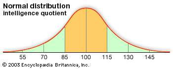
It has familiar bell-shaped curve is ubiquitous in statistical reports, from survey analysis and quality control to resource allocation.

The graph of the normal distribution is characterized by two parameters: the mean, or average, which is the maximum of the graph and about which the graph is always symmetric; and the standard deviation, which determines the amount of dispersion away from the mean. A small standard deviation (compared with the mean) produces a steep graph, whereas a large standard deviation (again compared with the mean) produces a flat graph.

1. The de Moivre–Laplace theorem is a special case of the central limit theorem, states that the normal distribution may be used as an approximation to the binomial distribution under certain conditions [2]. In particular, the theorem shows that the probability mass function of the random number of "successes" observed in a series of n independent Bernoulli trials, each having probability p of success (a binomial distribution with n trials), converges to the probability density function of the normal distribution with mean np and standard deviation

as n grows large, assuming p is not 0 or 1.

As n grows large, for k in the neighborhood of np we can approximate

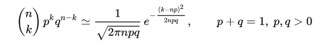
in the sense that the ratio of the left-hand side to the right-hand side converges to 1 as n → ∞.

The theorem appeared in the second edition of The Doctrine of Chances by Abraham de Moivre, published in 1738. Although de Moivre did not use the term "Bernoulli trials", he wrote about the probability distribution of the number of times "heads" appears when a coin is tossed 3600 times.

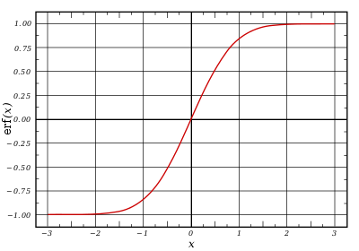
2. The Gauss error function), often denoted by erf, is a complex function of a complex variable defined as [3]:

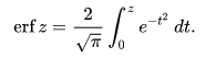
This integral is a special (non-elementary) and sigmoid function that occurs often in probability, statistics, and partial differential equations. In many of these applications, the function argument is a real number. If the function argument is real, then the function value is also real.

In statistics, for non-negative values of x, the error function has the following interpretation: for a random variable Y that is normally distributed with mean 0 and variance 1/2, erf x is the probability that Y falls in the range [−x, x].

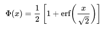
The error function is essentially identical to the standard normal cumulative distribution function [5]:

The two functions are closely related, namely

3. The Laplace distribution is a continuous probability distribution named after Pierre-Simon Laplace [4]. It is also sometimes called the double exponential distribution, because it can be thought of as two exponential distributions (with an additional location parameter) spliced together back-to-back, although the term is also sometimes used to refer to the Gumbel distribution. The difference between two independent identically distributed exponential random variables is governed by a Laplace distribution, as is a Brownian motion evaluated at an exponentially distributed random time. Increments of Laplace motion or a variance gamma process evaluated over the time scale also have a Laplace distribution.

Here, μ is a location parameter and b > 0, which is sometimes referred to as the diversity, is a scale parameter. If μ = 0 and b = 1, the positive half-line is exactly an exponential distribution scaled by 1/2.

The probability density function of the Laplace distribution is also reminiscent of the normal distribution; however, whereas the normal distribution is expressed in terms of the squared difference from the mean μ, the Laplace density is expressed in terms of the absolute difference from the mean. Consequently, the Laplace distribution has fatter tails than the normal distribution.

History [6, 7]. Some authors attribute the credit for the discovery of the normal distribution to de Moivre, who in 1738 published in the second edition of his "The Doctrine of Chances" the study of the coefficients in the binomial expansion of (a + b)^n. De Moivre proved that the middle term in this expansion has the approximate magnitude of 2/sqrt(2πn), and that "If m or ½n be a Quantity infinitely great, then the Logarithm of the Ratio, which a Term distant from the middle by the Interval ℓ, has to the middle Term, is −2ℓℓ/n. Although his theorem can be interpreted as the first obscure expression for the normal probability law, Stigler points out that de Moivre himself did not interpret his results as anything more than the approximate rule for the binomial coefficients, and in particular de Moivre lacked the concept of the probability density function.

In 1809 Gauss published his monograph "Theoria motus corporum coelestium in sectionibus conicis solem ambientium" where among other things he introduces several important statistical concepts, such as the method of least squares, the method of maximum likelihood, and the normal distribution. Gauss used M, M′, M′′, ... to denote the measurements of some unknown quantity V, and sought the "most probable" estimator of that quantity: the one that maximizes the probability φ(M − V) · φ(M′ − V) · φ(M′′ − V) · ... of obtaining the observed experimental results. In his notation φΔ is the probability law of the measurement errors of magnitude Δ. Not knowing what the function φ is, Gauss requires that his method should reduce to the well-known answer: the arithmetic mean of the measured values. Starting from these principles, Gauss demonstrates that the only law that rationalizes the choice of arithmetic mean as an estimator of the location parameter, is the normal law of errors:

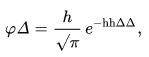
where h is "the measure of the precision of the observations". Using this normal law as a generic model for errors in the experiments, Gauss formulates what is now known as the non-linear weighted least squares (NWLS) method.

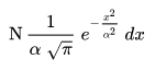
Although Gauss was the first to suggest the normal distribution law, Laplace made significant contributions. It was Laplace who first posed the problem of aggregating several observations in 1774, although his own solution led to the Laplacian distribution. It was Laplace who first calculated the value of the integral ∫ exp(−t^2) dt = √π in 1782, providing the normalization constant for the normal distribution. Finally, it was Laplace who in 1810 proved and presented to the Academy the fundamental central limit theorem, which emphasized the theoretical importance of the normal distribution. It is of interest to note that in 1809 an Irish mathematician Adrain published two derivations of the normal probability law, simultaneously and independently from Gauss. His works remained largely unnoticed by the scientific community, until in 1871 they were "rediscovered" by Abbe.

In the middle of the 19th century Maxwell demonstrated that the normal distribution is not just a convenient mathematical tool, but may also occur in natural phenomena: "The number of particles whose velocity, resolved in a certain direction, lies between x and x + dx is

---

References

1. https://www.britannica.com/topic/normal-distribution

2. https://en.wikipedia.org/wiki/De_Moivre%E2%80%93Laplace_theorem

3. https://en.wikipedia.org/wiki/Error_function

4. https://en.wikipedia.org/wiki/Laplace_distribution

5. https://en.wikipedia.org/wiki/Normal_cumulative_distribution_function

6. https://www.maa.org/sites/default/files/pdf/upload_library/22/Allendoerfer/stahl96.pdf

7. https://en.wikipedia.org/wiki/Normal_distribution#History